Intro
This Jupyter notebook describes the nflmodel Python package which can be used to predict the full probability distribution of NFL point-spread and point-total outcomes.
The model is inspired by the Elo based sports analytics work at fivethirtyeight.com and makes use of a machine learning algorithm that I developed called the margin-dependent Elo (MELO) model.
I describe the theory behind the algorithm at length in an arXiv pre-print, and you can also read about it on the MELO sphinx documentation page. The purpose of the blog post is not to rehash the theory behind the model, but rather to demonstrate how it can be used effectively in practice.
Requirements
The nflmodel package requires Python3 and is intended to be used through a command line interface. I've tested the package on Arch Linux and OSX, but not on Windows.
The model also requires an active internet connection to pull in the latest game data and schedule information. I'm working to enable offline capabilities, but this does not exist at the moment.
Installation
Navigate to the parent directory where you want to save the nflmodel package source, then run the following from the command line to install.
!git clone https://github.com/morelandjs/nfl-model.git nflmodel
!pip3 install --user nflmodel/.
After installing the nflmodel package, you'll need to populate the database of NFL game data. Since this is presumably your first time running the package, it will download all available games dating back to the 2009 season.
!nflmodel update
Subsequent calls to nflmodel update will incrementally refresh the database and pull in all new game data since the last update. If at any point your database becomes corrupted, you can rebuild it from scratch using the optional --rebuild flag.
Now that we've populated the database, let's inspect some of the game data contained within.
!nflmodel games
Each row corresponds to a single game, and each column is a certain attribute of that game. At the moment I populate the following attributes:
- datetime - (datetime64) - game start time
- season (int) - year in which the season started
- week (int) - nfl season week 1–17
- team_home (string) - home team city abbreviation
- qb_home (string) - home team quarterback name, first initial dot surname
- score_home (int) - home team points scored
- team_away (string) - away team city abbreviation
- qb_away (string) - away team quarterback name, first initial dot surname
- score_away (int) - away team points scored
Note, the nflmodel games runner is printing a pandas dataframe, so it may hide columns in order to fit the width of your terminal window. If you want to see more column output, try enlarging your terminal window.
If you want to see more row output, use the --head and --tail commands. For example,
!nflmodel games --head 3
The games dataframe is sorted from oldest to most recent, so --head N returns the N oldest games in the database and --tail N returns the N most recent games. If you want to print the entire dataset to standard out, just set --head or --tail to a very large number.
Calibration
The model predictions depend on a handful of hyperparameter values that are unknown a priori. These hyperparameters are:
- kfactor (float) - prefactor multiplying the Elo rating update; a larger kfactor makes the ratings more reponsive to game outcomes
- regress_coeff (float) - fraction to regress each rating to the mean after 3 months inactivity
- rest_bonus (float) - prefactor multiplying each matchup's rest difference (or sum)
- exp_bonus (float) - prefactor multiplying each matchup's quarterback experience difference (or sum)
- weight_qb (float) - coeficient used to blend team ratings and quarterback ratings.
Home field advantage is accounted for naturally by the MELO model constructor, so it is not included in the above list.
The hyperparameter values are calibrated by the following command (this will take several minutes or so, so grab a drink).
!nflmodel calibrate --steps 200
Here the argument --steps (default value 100) specifies the number of calibration steps used by hyperopt to optimize the hyperparameter values. I've generally found that around 200 calibration steps is sufficient, but the convergence is already very good after only 100 steps.
Note, the MELO model is actually very fast to condition once the hyperparameter values are known, so default behavior is to condition the model every time it is queried from the CLI. This ensures that the model predictions are always up to date.
Weekly forecasts
Once calibrated, the nflmodel package can forecast various metrics for a given NFL season and week. For instance, the command
!nflmodel forecast 2019 10
will generate predictions for the 10th week of the 2019 NFL season, using all available game data prior to the start of that week. If you do not provide the year and week, the code will try to infer the upcoming week based on the current date and known NFL season schedule.
The output is structured relative to the favorite team in each matchup, with home teams indicated by an '@' symbol. For example, the forecast output above says that NO is playing at home versus ATL, where they have a 91% win probability, are favored by 10 points, and are predicted to combine for 47.9 total points. The games are also sorted so that the most lopsided matchups appear first and most even matchups appear last.
Team rankings
The model will also provide team rankings at a given moment in time. For example, suppose I want to rank every team at precisely datetime = 2019-11-11T20:23:06. I can issue the command
!nflmodel rank --datetime "2019-11-11T20:23:06"
and see how the model thinks the teams should be ranked at that moment in time, according to their predicted performance against a league average opponent on a neutral field. The far left column is each team's predicted win probability, the middle column is its predicted Vegas point spread, and the far right column is its predicted point total.
The table above, for instance, tells me that BAL is most likely to win a generic matchup, while NE is most likely to blow out their opponent, and KC is the most likely to find itself in a shoot out.
Individual game predictions
One attractive feature of the MELO base estimator is that it predicts full probability distributions. This enables the model to do all sorts of cool things like predict interquartile ranges for the point spread or draw samples of a matchup's point total distribution.
Most notably, it means that the model can estimate the probability that the point spread (or point total) falls above or below a given line. This means that it can evaluate the profitability of various bets point spread and point total lines.
This capability is accessed using the nflmodel predict entry point. For example, suppose you want to analyze the game 2019-12-01 CLE at MIA with the following betting profile
| SPREAD | TOTAL | |
|---|---|---|
| CLE | -9.5 (-110) | O 46.5 (-105) |
| MIA | +9.5 (-110) | U 46.5 (-115) |
This is accomplished by calling the nfl predict runner with the following arguments.
!nflmodel predict "2019-12-01" CLE MIA --spread -110 -110 9.5 --total -105 -115 46.5
There's a lot of information here, so let's unpack what it means. First, the model believes CLE is a heavy favorite on the road. CLE's predicted win probability is 67%, their predicted point spread is -12.4 points, and their predicted point total is 44.9 points (according to the model). This would correspond to a characteristic final score of 29-16 CLE over MIA with fairly large uncertainties.
The model is also providing input on the Vegas point spread and point total lines. It expects CLE to cover their point spread line 58% of the time which is good for a 12% ROI, accounting for the house cut. Conversely, betting on MIA is expected to net a loss of 22% on average.
The over/under metrics are reported in a similar fashion. The model thinks there's a 53% chance the total score goes under the published Vegas line which results in a -1% loss on average. Similarly, taking the over is expected to net an 8% loss.
Quarterback changes
While it has not been readily apparent up to this point, the model accounts for changes at the quarterback position. It does this by tracking ratings at both the team and quarterback level.
For example, suppose Tom Brady were the only quarterback that ever played for the Patriots. Then there would be two associated ratings, one for T.Brady and one for NE, which are effectively identical. If however, Tom Brady left NE and went to play for SF for the last two years of his career, his rating would diverge from NE's rating and begin to track the performance of SF.
I take the weighted average of QB level and team level ratings when generating the effective rating for each upcoming game. In this way, I mix together the historical performance of the team with its QB. The weighted average is controlled by the qb_weight hyperparameter which is fixed when calibrating the model.
The model has no direct knowledge of QB injuries, so you'll have to explicitly tell the model to generate predictions with a different quarterback if that's what you intend to do. At the moment, the only runner that can accommodate QB injuries is the nflmodel predict runner.
Suppose, for example, you want to see how CLE would perform on the road against PHI on 2019-12-01 if Carson Wentz went out with an injury practicing before the game. First let's see how the two teams would matchup if Wentz never got hurt.
!nflmodel predict "2019-12-01" CLE-B.Mayfield PHI-C.Wentz
Notice that the predictions are exactly the same if I omit the quarterback suffixes.
!nflmodel predict "2019-12-01" CLE PHI
This is because both Baker Mayfield and Carson Wentz played in the game preceding the specified date, so the model assumes they are the starting QBs for upcoming games by default.
Suppose now, that Wentz got hurt. We can specify his backup QB Josh McCown to see how that would affect the model predictions.
!nflmodel predict "2019-12-01" CLE PHI-J.McCown
This creates roughly a 7 point swing in the point spread and CLE is now the favorite. In fairness to Josh McCown, the magnitude of this point shift is not purely a statement about the better QB. It also accounts for the fact that PHI has not been game planning for McCown, and the offense is not built around him.
Validation
The nflmodel package includes a command line runner to validate the predictions of the model. If the model predictions are statistically robust, then the distribution of standardized residuals will be unit normal and the distribution of residual quantiles will be uniform.
This is a very powerful test of the model's veracity, but it does not necessarily mean the model is accurate. Rather it tests whether the model is correctly reporting its own uncertainties. To quantify the model's accuracy, nflmodel validate also reports the models mean absolute prediction error for seasons 2011 through present.
!nflmodel validate
This will produce two figures, validate_spread.png and validate_total.png in the current working directory. For example, the point spread validation figure is shown below.
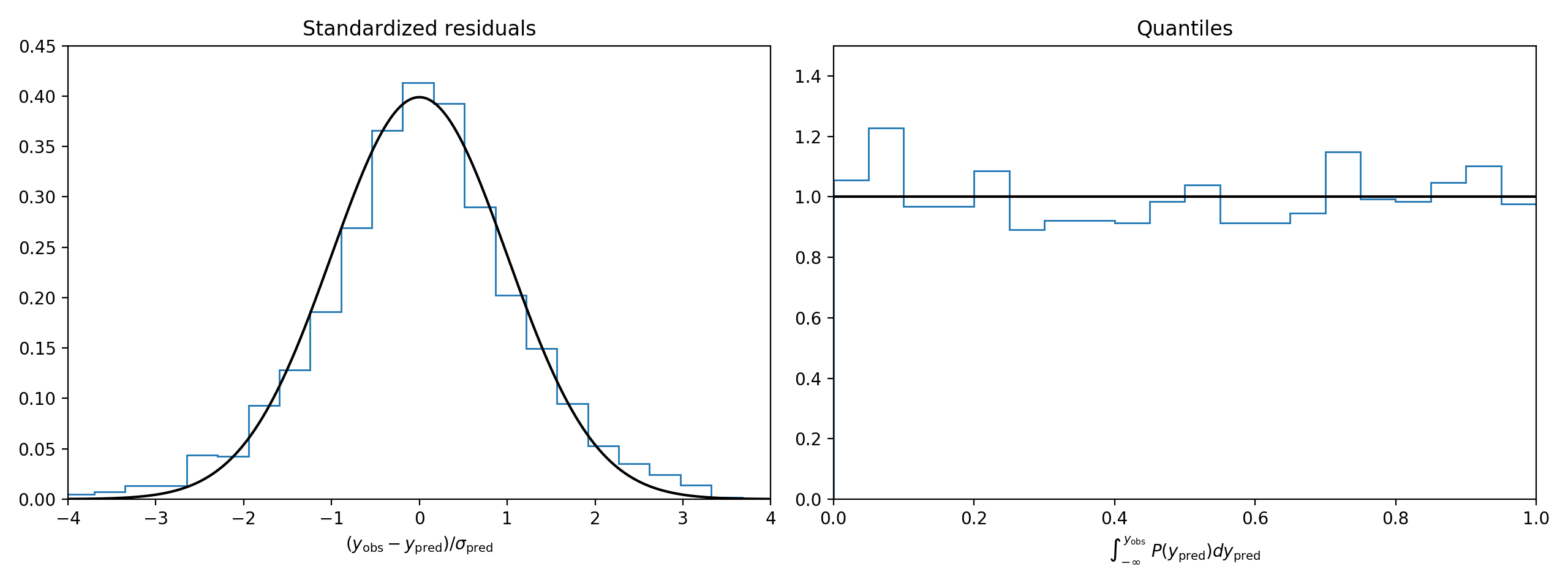
The model's point spreads have a mean absolute error of 10.37 points and its point totals have a mean absolute error of 10.70 points. The table below compares the model's point spread mean absolute error to Vegas for the specific season range 2011–2019.
| MAE | SPREAD | TOTAL |
|---|---|---|
| MODEL | 10.37 pts | 10.70 pts |
| VEGAS | 10.23 pts | 10.49 pts |
The model is less accurate than Vegas, but these numbers are still promising considering that many factors remain missing from the model such as weather and personnel changes.
Betting simulation
I've also bundled a small script nflmodel/tutorial/simulate-bets.py inside the tutorial directory which can simulate the performance of the model as a betting tool on historical games. Hereafter, I restrict my attention to point spreads since I'm currently neglecting many factors which are specifically important to point total values like stadium type and weather.
The general idea is as follows. I backtest the model and estimate the probability that the home team and away team each cover their Vegas spread (scraped from covers.com) at the moment just before kickoff. If the model believes that either team will cover their spread with a likelihood greater than X, where X is a fixed decision threshold, then I place a simulated bet on that team.
When the threshold X=50%, the simulation places bets on every game, and when the threshold X ≫ 50%, the simulation is far more selective with the games it chooses to bet on. If I set the decision threshold X > 90% then the model cannot find any games with sufficiently high confidence to bet on.
In principle, one expects the model to get more bets correct when X is large because it is more confident in those bets. The goal here is to see if there is a threshold X which is sufficiently large to yield a positive ROI.
Technically, I need more information to compute the model's ROI than just the historical spread. I also need the vigorish or "juice" on each spread which is the cut taken by the house in order to place a bet. Typically this ranges anywhere from -100 to -120 for spread bets, which means you might need to risk up to 120 dollars in order to win 100 dollars. More extreme vigs exist but they are uncommon.
Unfortunately, I do not have the historical vigs for these lines, precluding a true ROI simulation. However, you can rest assured that the ROI will be strongly negative if the model is not getting more games right than wrong. So for now, let's just see if I can demonstrate that the model is better than 50-50 with statistical significance.
Statistical significance here is key. As I increase the betting threshold, I reduce my validation statistics because the number of qualifying games drops. For large values of the threshold X, the model may only find a dozen or so qualifying games to bet on. This means the results of the simulation will be noisy and it will be possible to be duped by statistical fluctuations (we've all seen someone flip four heads in a row).
To calculate statistical significance, I compute the 90% interquartile range for the null model, i.e. the range of reasonable outcomes for independent random wins sampled with 50% probability. In other words, I compare my model's success rate to what one would expect from random chance.
The results of this calculation are shown below for a decision threshold X=0.8.
!python3 simulate-bets.py 0.8
Here we see that the model is performing at the ~90% quantile level, i.e. not something you'd use to bet a ton of money, but I think impressive nonetheless.
Who's going to win Super Bowl LIV?
Unfortunately, I have not prepped the model to work on the post-season yet. There's nothing that precludes applying the model to the post-season, it just involves some more work, and I haven't had time to do it yet.
In any event, I think this tutorial shows that the Vegas lines are quite accurate, and it is non-trivial to build a model that beats them. The small number of available games makes NFL modeling a uniquely interesting problem, and I've learned quite a bit on my own quest to build a better model.
Please feel free to contact me at morelandjs@gmail.com with questions and comments.
Thank you!
-Scott